A Close Reading of Self-Attention

This article assumes comfort with linear algebra. It’s designed for those who have seen the self-attention formula but haven’t yet found the time to really understand it (i.e., me).

Self-attention is a mechanism in deep learning that allows positions in sequences to aggregate information from other positions of their ‘choosing’, depending on the specific input. We’ll make this intuition precise.

For starters, self-attention is a sequence-to-sequence map. Each element of the output sequence is a weighted average of feature vectors, where the weights and feature vectors are determined from the input sequence.

Mathematically: Self-attention maps an $S$-element sequence of $d$-vectors, $x \in \mathbb{R}^{S \times d}$, to another $S$-element sequence of $d_v$-vectors, $\text{Attention}(x) \in \mathbb{R}^{S \times d_v}$. Its elements are given by $$\text{Attention}(x)_{i} = A_{i}V = \sum_{j} A_{ij} V_j,$$for a weight matrix $A$ whose rows $A_i$ sum to one: $\sum_j A_{ij} = 1$. The $i$th output vector is the weighted average of feature vectors $V_{j} \in \mathbb{R}^{d_v}$.

Feature vectors, $V$

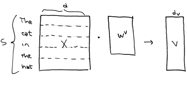
The feature vectors are a linear projection of the input. For an input sequence $x \in \mathbb{R}^{S \times d}$, the feature matrix $V \in \mathbb{R}^{S \times d_{v}}$ is $$V = xW^V,$$ for some low-dimensional projection matrix $W^V \in \mathbb{R}^{d \times d_{v}}$. Think of $V$ as a batched projection of $x$, so each sequence element is passed through the same projection.

Attention matrix, $A$

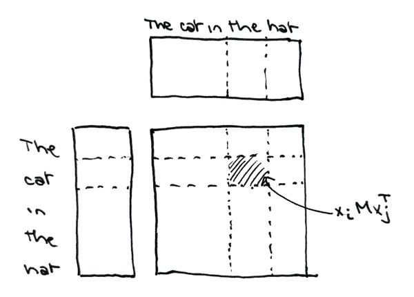
The ‘weight’ matrix $A \in \mathbb{R}^{S \times S}$ is a normalized similarity matrix, where each entry $A_{ij}$ represents a measure of “alignment” between $x_{j}$ and $x_{i}$. Alignment is measured through the kernel matrix,$$xMx^T,$$for some learnable matrix $M \in \mathbb{R}^{d \times d}$. Each element $ij$ represents the dot product (in the geometry defined by $M$) between input vectors $x_i$ and $x_j$. The matrix $M$ may be asymmetric, so$$(xMx^T)_{ij} \neq (xMx^T)_{ji},$$in general.

The attention matrix $A$ is constructed by passing this kernel matrix through an element-wise nonnegative function $\psi$, then normalizing each row to have unit sum. Specifically, $$A_{ij} := \frac{\psi(x_{i}Mx_{j}^T)}{\sum_{k} \psi(x_{i}Mx_{k}^T)}$$ In practice, $\psi$ is often chosen to be $\psi = \text{exp}$.¹ With this choice, $A$ can be concisely expressed as the result of a softmax operation applied rowwise: $$A = \text{softmax}_{\text{rowwise}}\left(xMx^T \right).$$

Convex combinations, $AV$

With $V$ and $A$ defined, we can pull together a precise understanding of self-attention.

Self-attention maps one sequence to another of the same length. Each element $\text{Attention}(x)_i$ in the output sequence is a convex combination of linear features $V$ of the input sequence $x$. $$\text{Attention}(x)_{i} = A_{i}V = \sum_{j} A_{ij}V_{j}$$ Each combination weight $A_{ij}$ is determined based on the kernel similarity between $x_i$ and $x_j$, normalized by its similarities to all other sequence elements.²

Parameterizing $M$

In practice, we don’t learn the bilinear form matrix $M$ directly. Instead, we constrain its rank (and hopefully make it easier to learn) by parameterizing as a product of lower-dimensional factors.

We pre-specify a maximum rank $d_k$, and parameterize $M$ in terms of learnable $d \times d_{k}$ matrices $W^Q, W^K$, as follows: $$M = \frac{1}{\sqrt{d_{k}}} (W^Q)(W^K)^T.$$ The product is scaled by $\frac{1}{\sqrt{ d_{k} }}$ to limit the magnitude of the entries in practice. The goal is to avoid pushing the softmax inputs into regions where the nonlinearity has very small gradients.

The usual notation

Translating from our expression $$\text{Attention}(x) = \text{softmax}_{\text{rowwise}}(xMx^T)V$$ to the form generally seen in papers, $$\text{Attention}(Q, K, V) = \text{softmax}_{\text{rowwise}}\left( \frac{QK^T}{\sqrt{ d_{k} }} \right)V$$ is quite simple.

To do so, we define the usual $Q, K$ matrices by “pulling” the factors $W^Q$ and $W^K$ onto each $x$ term in the kernel matrix computation. Specifically, define $Q, K \in \mathbb{R}^{S \times d_{k}}$ as $$Q = xW^Q \quad \text{and} \quad K = xW^K,$$ Like with the projection matrix $W^V$ above, this operation is best understood as a “batched projection.” The two notations are then trivially equivalent, with$$xMx^T = x \left( \frac{1}{\sqrt{ d_{k} }} (W^Q) (W^K)^T \right)x^T = \frac{1}{\sqrt{ d_{k} }} (xW^Q)(xW^K)^T = \frac{1}{\sqrt{ d_{k} }}QK^T.$$All together:$$\text{Attention(x)} = AV = \text{softmax}(xMx^T)V = \text{softmax}\left( \frac{QK^T}{\sqrt{d_{k} }} \right) V.$$

So what?

Abstractly, this article frames self-attention as the composition $$\text{Attention}(x)_{i} = \big[ \text{Normalize}(\text{Kernel}(x_{i}, x)) \big] \text{Features}(x).$$ In words, self-attention computes an output sequence where each element $i$ is a convex combination of feature vectors $j$. The contribution of vector $j$ to the output (the magnitude of its combination weight, $A_{ij}$) is determined by a normalized kernel similarity between input elements $i$ and $j$.

This framing makes apparent some otherwise hand-wavy observations.

Observation 1: Self-attention reduces the ‘distance’ between tokens $i$ and $j$

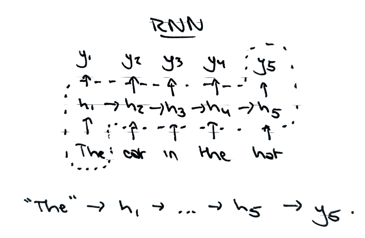
Self-attention is a powerful mechanism because it calculates each output element $i$ by directly pulling information from other tokens $j$. Compare this to the dependency between tokens in a recurrent neural network. Define the basic RNN as $$\text{RNN}(x)_{t} := g(h_{t}) \quad \text{and} \quad h_{t} := f(x_{t}, h_{t - 1}).$$ Each output computed, $\text{RNN}(x)_{i}$, is the result of $i$ recursive applications of $g$ and $f$ along the input sequence. The information about early tokens $x_1, ..., x_i$ is bottlenecked through the single “hidden state” representation $h_i$.

In theory, $h_i$ should be able to represent all the relevant information from the previous sequence tokens. But in practice, RNNs don’t learn to compress this information well.³

Self-attention sidesteps this compression problem. It removes the hidden state bottleneck and directly mixes features from other tokens.

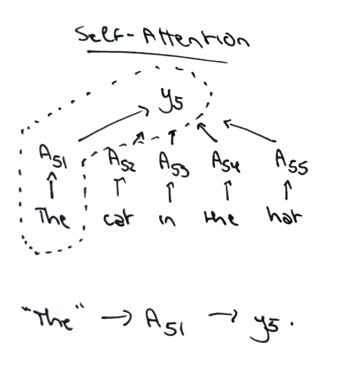In doing so, self-attention also parallelizes the sequence-to-sequence computation.

RNNs are inherently sequential, since their output at time $t+1$ depends on the previous hidden state $h_t$. But with self-attention, each output term $\text{Attention}(x)_{i}$ and $\text{Attention}(x)_{j}$ can be computed completely in parallel.

This parallelization, however, does come at a cost.

Observation 2: Self-attention has no “interaction terms”

Because self-attention parallelizes the similarity computation for output $i$ across all input elements $j$ at once, it’s quite restricted in the way it can combine information from input tokens.

Specifically, self-attention can only ‘combine’ information from tokens $j, k$ into $\text{Attention}(x)_{i}$ through the linear mixing $$A_{ij}V_{j} + A_{ik}V_{k}.$$ Even the linear mixing weights $A_{ij}$ and $A_{ik}$ depend largely only on the individual similarities $\text{Kernel}(x_i, x_{j})$ and $\text{Kernel}(x_i, x_{k})$. This turns out to limit the kinds of computations that (a single layer of) self-attention can perform.⁴

Various generalizations of self-attention aiming to address this limitation by incorporating interaction terms have been proposed.

The basic concept of “higher-order attention” is simple, and fits nicely into the framework we’ve discussed. For concreteness, let’s consider third-order attention.⁵

Third-Order Attention

There are two key changes. Rather than mixing individual features $V_j$ associated with individual tokens $x_j$, we mix pair features $V_{j, k}$ associated with token pairs $x_{j, k}$. Rather than defining the mixing weights for output $i$ using the similarity between $x_{i}$ and all other tokens $x_{j}$, we mix the pair features based on the similarity between $x_i$ and all pairs of tokens $x_j, x_k$.

The final form of third-order attention is semantically equivalent to standard attention. It composes an output sequence composed by linearly mixing interaction features from the input: $$\text{Attention}_{3}(x)_{i} = \sum_{j, k}\big[ \text{Normalize}(\text{Kernel}(x, x, x)) \big]_{i, j, k} \text{Features}_{j,k}(x)$$ Recent research has demonstrated practical performance improvements from incorporating higher-order attention layers (Roy et al, 2025).

But unfortunately, there are no free lunches. Higher-order attention is significantly more expensive. Whereas standard self-attention is $O(S^2)$, third-order attention is $O(S^3)$, since we now need to compute an $S \times S \times S$ attention tensor rather than an $S \times S$ attention matrix.

Conclusion

We’ve now thoroughly examined each component of self-attention. The self-attention mechanism is a sequence-to-sequence transformation that computes each output as a weighted average of features, where the weights are based on normalized similarities between input sequence elements. This framing precisely undergirds the intuition that self-attention allows positions to “look at” and “choose” information from other positions.

---